Lane Keeping RC Car

Introduction

During my final semester at Cal, I took ME131: Vehicle Dynamics and Control. The course focused on modeling automotive vehicle dynamics, understanding instabilities and safety implications, then building controllers to improve the vehicle behavior somehow. Modern cars have a slew of feedback control laws running at all times. We might segment all these controllers into two groups:

1. Low Level Controllers

Low level controllers augment the vehicle’s dynamics to enhance safety or performance. They run at all times in normal passenger cars and they all work to ensure that the tires don’t exceed their friction limits. These include (but are certainly not limited to):

• Anti-lock braking systems (ABS): modulates braking force to ensure the tires do not exceed their friction limits under maximum vehicle deceleration.
• Traction control: modulates engine torque to ensure the tires do not exceed their friction limits under maximum vehicle acceleration.
• Electronic stability control (ESP): is usually implemented as differential braking between the left and right wheels to control the yaw rate of the vehicle while turning.

2. High Level Controllers

High level controllers relieve the driver of some part of the driving task. These controllers are meant to be a convenience to the driver. I’ve listed them in order of increasing sophistication and autonomy:

• Cruise control: modulates engine torque to maintain a desired reference speed.
• Adaptive cruise control: modulates engine torque and braking force to maintain a desired speed or following distance to the car ahead.
• Lane keep assist: actuates the car’s steering to maintain a position inside the lane, often combined with adaptive cruise control for autonomous highway driving (such as the current state of Tesla’s “autopilot”).

The automotive world offers an extremely rich area of study for controls engineering, and now more than ever as ubiquitous sensors and compute find their way into modern vehicles. The massive effort for fully autonomous driving in the industry today makes automotive controls even more compelling. In ME131 I had the chance to derive and simulate vehicle dynamics in Matlab, then implement controllers I designed on a 1/10th scale RC car called the Berkeley Autonomous Racecar (BARC). Let’s talk about the robot itself first.

The BARC

The BARC was developed by the MPC Lab at UC Berkeley. It is a 1/10th scale, all-wheel-drive electric racecar. More information on the BARC project, including a bill of materials is available here.

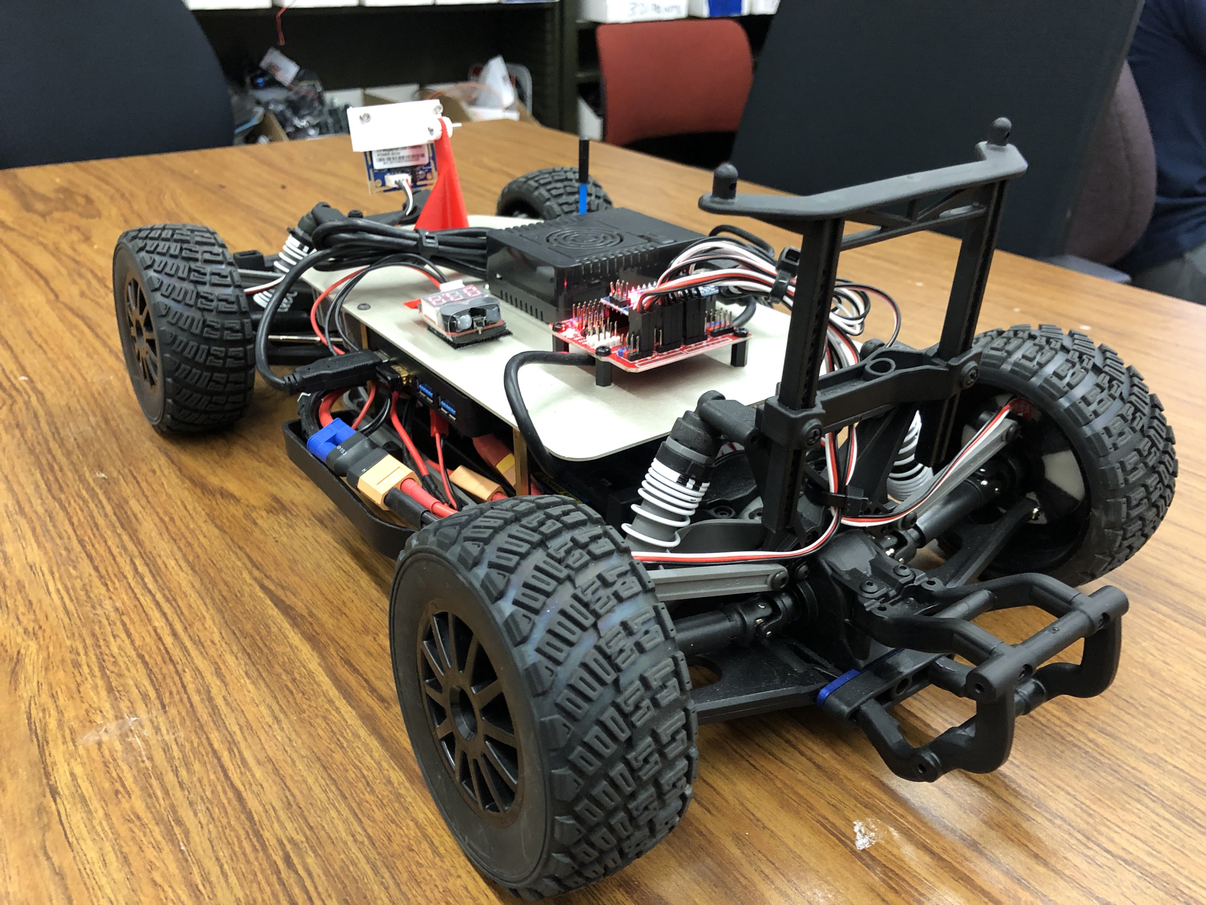
Powertrain

The vehicle is powered by a 2S, 8 Ah lithium-polymer battery. The drivetrain includes an electronic speed controller (ESC) which converts DC power from the battery to 3-phase AC for the brushless motor. The ESC also contains a 5V battery eliminator circuit (BEC) and serves as power distribution for the steering servo.

Sensors

The BARC features an optical encoder on each wheel with eight counts per wheel revolution, allowing for an angular velocity estimate of each wheel. It also features a front facing digital camera which communicates data over serial to an ebedded Linux computer for processing at 30 frames per second. Color or intensity gradient thresholding on the image stream from the camera allows for edge detection within these frames, and thus for semantic data regarding relative position of the vehicle to a lane, to be extracted. The BARC also features an inertial measurement unit (IMU) consisting of an accelerometer and rate gyroscope for measurement of proper acceleration and angular rates of the vehicle. The IMU is not utilized in our lane keeping experiment.

Compute

High level processes are handled by an Odroid XU4 embedded Linux computer running an image of Ubuntu Mate 16.04 maintained by the Berkeley MPC Lab. The Odroid has a 2Ghz ARM-based processor and 2Gb of DDR3 RAM making it a capable platform for soft real-time applications. The Odroid has several I/O ports and publishes a wifi access point for wireless communication with a host computer via secure shell (SSH) or virtual network computing (VNC). Low level processes are handled by an Arduino Nano microcontroller. This device reads sensor data and relays the data over serial to the Odroid. The microcontroller also receives control commands over serial from the Odroid and communicates via pulse width modulation (PWM) with the ESC. Several of these components are labeled in the image below.

Software

The Robot Operating System (ROS) is heavily used for inter-process communication onboard the BARC. ROS Kinetic is installed with the MPC lab’s distribution of Ubuntu Mate 16.04 for the Odroid. Processes are segmented into nodes which publish and/or subscribe to topics on which messages of a given data structure are communicated. Often nodes are associated with hardware interfaces, data processing, controllers, estimators, etc. The data processing, estimators, and controllers for the lane keeping system are implemented in python leveraging several open source libraries including OpenCV and controlPy.

Lane Keeping

Dynamics

Vehicle dynamics is a complicated subject, people get doctorates in it. Mostly these complications arise due to the nature of tire/road interactions. If I learned one thing from ME131 its that “tires are complicated.” Tires exert a force on the road through the viscoelastic deformation of the contact patch that the rubber of the tire forms on the road. Material properties of the rubber and of the ground are necessary to make an any detailed predictions about the force a tire will exert on the road. Several models, with different physical intuitions, exist and are used commonly in industry (see Dougoff and Pacejka tire models). To avoid these complications (and because the tires on the BARC are made of hard plastic), we’ll leave tire force terms unexpanded, or relate them directly to motor torque.

Longitudinal Dynamics

The longitudinal dynamics (aligned with the forward direction of the vehicle) can be expressed easily via Newton’s second law.

$F_{x_F}$ and $F_{x_R}$ are the front and rear tire forces exerted on the vehicle to propel it forward. $F_{aero}$ is aerodynamic drag. $R_{x_F}$ and $R_{x_R}$ are the front and rear tire rolling resistances. And $mg\sin{\theta}$ is the component of gravitational acceleration pulling the vehicle down an incline of angle $\theta$.

We can be more specific about $F_{aero}$ if we like:

• $\rho$ is the mass density of the air
• $C_d$ is the drag coefficient of the vehicle (as determined via CFD, wind tunnel, or full scale testing)
• $A_F$ is the front area of the vehicle, the area of the vehicle that the oncoming wind “sees”
• $v_x$ and $v_{wind}$ are the longitudinal velocity of the vehicle and the headwind velocity if one exists.

Lateral Dynamics

Lateral dynamics are significantly richer than longitudinal dynamics. There’s two approaches we can take here, the more accurate but more complicated approach would be to study forces and torques on the vehicle due to tire/road interactions, assuming we have a tire model we’re comfortable with. A large simplification we can make for a limited set of driving conditions is called the “kinematic bicycle model.” This approach is “kinematic” because we’ll ignore forces and torques and use only geometric constraints to derive the equations of motion of the vehicle. Its called a “bicycle” model because we’ll combine the left and right tires into one entity each such that the vehicle has two wheels, a front and back, just like a bicycle:

• $x$ is the inertial x coordinate
• $y$ is the inertial y coordinate
• $v$ is the longitudinal velocity of the vehicle
• $\psi$ is the heading angle of the vehicle in the inertial frame
• $\delta_f$ is the steering angle of the front wheels
• $l_r$ is the distance from the vehicle’s center of mass to the rear axle
• $l_f$ is the distance from the vehicle’s center of mass to the front axle
• $\beta$ is the sideslip angle (the angle between the vehicle’s velocity vector and its longitudinal axis)

The state variables will be $z = [x, y, \psi]^T$ and the inputs will be $u = [v, \delta_f]^T$.

We’re making two critical assumptions when we use the kinematic bicycle model.

1. The velocity vectors at the front and rear tires are parallel to the direction of the tires, i.e. there are no lateral tire forces.

2. The radius of the vehicle path changes slowly such that $\dot{\psi} = \frac{v}{r}$ holds.

These assumptions make our model appropriate for slow speed driving (as in a parking lot rather than on a freeway). As a visual representation of this limitation, we can compare the open loop performance of the kinematic model to predict the motion of a vehicle to the performance of a more sophisticated dynamic model which does take tire forces into account. I was given differential GPS data for a vehicle performing a severe figure-8 maneuver. I implemented both the kinematic bicycle model shown above and a dynamic bicycle model in Simulink, and using the recorded longitudinal velocity and steering angle off the vehicle, simulated both models to see how quickly they diverged off the dGPS truth. Check out the code here.

LQR Steering Controller

The steering controller exists in a script called $\texttt{LQR_synth.py}$ which you can find here. We use a discrete-time, infinite-horizon linear quadratic regulator (LQR) approach which minimizes a cost associated with state error and control effort. The script is a ROS node which subscribes to an estimate of the track radius, a vehicle velocity estimate, the previous loop’s steering command, and the loop time $dt$ in order to compute an LQR gain matrix $K(t)$ at each loop. A Jacobian linearization of the nonlinear kinematic model is computed as an input to the Riccati solver in the controlPy python toolbox (controlPy was incidentally built by my old PI from the HiPeRLab). Because a new gain matrix is computed at loop rather than computing one gain matrix to use for all operating conditions, we’ll call the controller a “gain-scheduled” LQR controller.

The script then computes the optimal control output and publishes it for the Arduino to send to the actuators. The controller must be able to handle non-static setpoints (the track curvature varies unpredictably with time) so we choose a reference tracking LQR controller which brings the error between estimated and reference states to zero. We also include a feedforward steering term computed directly by the kinematic bicycle model. The full gain scheduled, reference tracking LQR lane keeping controller with feedforward can be represented as:

Where $K(t)$ is the time varying LQR gain matrix, $z(t) - z_{ref}(t)$ is the state error, and $u_{ref}(t)$ is the feedforward term from the kinematic bicycle model.

Demo

Results

The problem of autonomous navigation is hard because it consists of several sub-problems which are difficult in their own right, and solutions to these problems must work in harmony to deliver a robust system. Perception, trajectory generation, and control modules must deliver simultaneously for reliable driving. Our system focused on the control aspects of the problem, and thus shortcuts were taken in the perception and trajectory generation steps which lead to most of the issues we debugged after implementing our algorithms. The lane localization system used a simple edge detection algorithm based on finding intensity gradients greater than a hard coded threshold. This approach is not robust to changes in lighting, texture, or reflectance of the driving surface. Our vehicle struggled to reliably find lanes on shiny floors so we found a large space with dark carpeting and used bright white tape as lane lines for maximum contrast which improved tracking performance.

I’m interested in continuing to build and experiment with small RC cars. They’re a relatively cheap way to get directly involved in the technology powering a future multi-billion dollar self-driving industry.

My code for the project is available on Github.